Pupil data pre-processing
pupil dilation, pupillometry, eye-tracking, experiments, infant research, DevStart, developmental science
Welcome to your first step into the world of pupillometry! In this tutorial, we’ll walk you through how to preprocess pupil data using a handy R package called PupillometryR. This package makes it simple to clean and even analyze your pupil data with just a few lines of R code.
To keep things straightforward, we’ll be working with a simulated dataset that you can download right here:
Download and unzip this folder. This dataset is based on the experimental design we introduced earlier in our eye-tracking series. If you’re not familiar with it or need a quick refresher, we recommend checking out the “Introduction to eye-tracking” guide before diving in.
This tutorial serves as a foundation for understanding how to preprocess pupil data. Once you’ve grasped the essentials, we encourage you to explore the full range of functions and features PupillometryR has to offer.
In this and upcoming tutorials, we’ll use dplyr, a package included in the tidyverse collection. dplyr is designed for efficient manipulation of dataframes and makes it easy to perform operations using the Magrittr pipe (%>%). This pipe allows you to chain multiple operations on a dataframe in a seamless flow, avoiding intermediate steps or temporary variables.
We’ll focus on basic dplyr functions for now, including:
filter(): Used to subset rows based on specific conditions.
Example: Keep rows wheredata %>% filter( Event == "Circle").mutate(): Adds or modifies columns in the dataframe.
Example: Create a new columndata %>% mutate(mean_pupil_norm = mean_pupil / 100).group_by(): Groups the dataframe by one or more columns for grouped operations.
Example: Group data bydata %>% group_by(Subject, Event).summarize(): Aggregates data within groups to compute summary statistics.
Example: Calculate the mean pupil size for each group.
Basic Syntax
The syntax begins by passing a dataframe into the pipe (%>%) and then applying one or more operations. These functions directly manipulate the dataframe without requiring it (or its columns) to be explicitly referenced in each step.
Here’s an example:
This code filters rows where Events == "Circle", groups data by Subject, and calculates the mean pupil size for each subject, creating a new dataframe, data2, in a concise and readable flow. 🚀
This is just the tip of the iceberg ❄️—dplyr is an incredible tool! If you want to explore its full potential, check out this tutorial: R dplyr Tutorial | Learn with Examples
Read the data
Let’s begin by importing the necessary libraries and loading the downloaded dataframe.
Great! Now, let’s locate and load all our data files. We’ll use list.files() to identify all the .csv files in our folder. Make sure to update the file path to match the location where your data is stored.
csv_files = list.files(
path = "..\\..\\resources\\Pupillometry\\RAW",
pattern = "\\.csv$", # regex pattern to match .csv files
full.names = TRUE # returns the full file paths
)csv_files is now a list containing all the .csv files we’ve identified. To better understand our dataset, let’s start by focusing on the first file, representing the first subject, and inspect its structure. This will give us a clear overview before we proceed further.
X Subject time L_P R_P Event TrialN
1 1 Subject_1 1.000000 3.187428 3.228510 Fixation 1
2 2 Subject_1 4.333526 3.153315 3.193957 <NA> NA
3 3 Subject_1 7.667052 3.102050 3.142032 <NA> NA
4 4 Subject_1 11.000578 3.163670 3.204446 <NA> NA
5 5 Subject_1 14.334104 3.152682 3.193316 <NA> NA
6 6 Subject_1 17.667630 3.086508 3.126289 <NA> NAOur dataframe consists of several easily interpretable columns. time represents elapsed time in milliseconds, Subject identifies the participant, and Event indicates when and which stimuli were presented. TrialN tracks the trial number, while L_P and R_P measure pupil dilation for the left and right eyes, respectively, in millimeters.
Let’s plot the data! Visualizing it first is always a crucial step as it provides an initial understanding of its structure and key patterns.
ggplot(Raw_data, aes(x = time, y = R_P)) +
geom_line(aes(y = R_P, color = 'Pupil Right'), lwd = 1.2) +
geom_line(aes(y = L_P, color = 'Pupil Left'), lwd = 1.2) +
geom_vline(data = Raw_data |> dplyr::filter(!is.na(Event)), aes(xintercept = time, linetype = Event), lwd = 1.3) +
theme_bw(base_size = 35) +
ylim(1, 6) +
labs(color= 'Signal', y='Pupil size')+
scale_color_manual(
values = c('Pupil Right' = '#4A6274', 'Pupil Left' = '#E2725A') ) +
theme(
legend.position = 'bottom' ) +
guides(
color = guide_legend(override.aes = list(lwd = 20)),
linetype = guide_legend(override.aes = list(lwd = 1.2))
)Prepare the data
Nice!! Now we have some sense of our data!! And….you’ve probably noticed two things:
So many events! That’s intentional — it’s better to have too many triggers than miss something important. When we recorded the data, we saved all possible events to ensure nothing was overlooked. But don’t worry, for our pupil dilation analysis, we only care about two key events: Circle and Square (check the paradigm intro if you need a refresher on why this is)
Single-sample events! Like in most studies, events are marked at a single time point (when the stimulus is presented). But PupilometryR needs a different structure — it expects the event value to be repeated for every row while the event is happening.
So, how do we fix this? First, let’s isolate the rows in our dataframe where the events are Circle or Square. We start by creating a list of the events we care about, then use it to filter our dataframe and keep only the rows related to those events in a new dataframe called Events
Events_to_keep = c('Circle','Square')
Events = filter(Raw_data, Event %in% Events_to_keep) # filter data
head(Events) # database peak X Subject time L_P R_P Event TrialN
1 221 Subject_1 734.3757 NA NA Circle 1
2 2552 Subject_1 8504.8248 3.596057 3.642405 Square 2
3 4883 Subject_1 16275.2739 3.543367 NA Circle 3
4 7215 Subject_1 24049.0565 3.164419 3.205205 Circle 4
5 9546 Subject_1 31819.5055 3.147494 3.188061 Square 5
6 11877 Subject_1 39589.9546 3.343493 3.386587 Circle 6Perfect! Now onto the second point: we need to repeat the events we just selected for the entire duration we want to analyze. But what’s this duration? We want to cover the full cue presentation (2 seconds), plus an extra 0.1 seconds before the stimulus appears. Why? This pre-stimulus period will serve as our baseline, which we’ll use later in the analysis.
So, let’s define how much time to include before and after the stimulus. We’ll also set the framerate of our data (300Hz) and create a time vector that starts from the pre-stimulus period and continues in steps of 1/Hz, with a total length equal to Pre_stim + Post_stim.
# Settings to cut events
Fs = 300 # framerate
Step = 1000/Fs
Pre_stim = 100 # pre stimulus time (100ms)
Post_stim = 2000 # post stimulus time (2000ms)
Pre_stim_samples = Pre_stim/Step # pre stimulus in samples
Post_stim_samples = Post_stim/Step # post stimulus in samples
# Time vector based on the event duration
Time = seq(from = -Pre_stim, by=Step, length.out = Pre_stim_samples+Post_stim_samples) # time vectorHere’s where the magic happens. We loop through each event listed in our Events dataframe. Each row in Events corresponds to a specific event (like a “Circle” or “Square” cue) that occurred for a specific subject during a specific trial.
For each event, we extract 2 key details:
Event (to know if it’s a Circle or Square cue)
TrialN (to know which trial this event is part of)
Next, we identify the rows of interest in our main dataframe. First, we locate the row where the time is closest to the onset of the event. Then, we select a range of rows that fall within the Pre_stim and Post_stim window around the event.
Finally, we use these identified rows to add the event information. The Time, Event, and TrialN values are repeated across all the rows in this window, ensuring every row in the event window is properly labeled.
# Loop for each event
for (trial in 1:nrow(Events)){
# Extract the information
Event = Events[trial,]$Event
TrialN = Events[trial,]$TrialN
# Event onset information
Onset = Events[trial,]$time
Onset_index = which.min(abs(Raw_data$time - Onset))
# Find the rows to update based on pre post samples
rows_to_update = seq(Onset_index - Pre_stim_samples,
Onset_index + Post_stim_samples-1)
# Repeat the values of interest for all the rows
Raw_data[rows_to_update, 'time'] = Time
Raw_data[rows_to_update, 'Event'] = Event
Raw_data[rows_to_update, 'TrialN'] = TrialN
}Perfect! We’ve successfully extended the event information backward and forward based on our Pre_stim and Post_stim windows. Now, it’s time to clean things up.
Since we only care about the rows that are part of our trial of interest —and because the event information is now repeated for each row during its duration— we’ll remove all the rows that don’t belong to these event windows. This will leave us with a clean, focused dataset that only contains the data relevant to our analysis.
For all subjects
Great job making it this far! Fixing the data to make it usable in PupillometryR is definitely one of the trickiest parts. But… we’ve only done this for one subject so far—oops! 😅 No worries, though. Let’s automate this process by putting everything into a loop for each subject. In this loop, we’ll fix the event structure for each subject, store each subject’s processed dataframe in a list, and finally combine all these dataframes into one single dataframe for further analysis. Let’s make it happen!
# Libraries and files --------------------------------------------------------------------
library(PupillometryR) # Library to process pupil signal
library(tidyverse) # Library to wrangle dataframes
library(patchwork)
csv_files = list.files(
path = "..\\..\\resources\\Pupillometry\\RAW",
pattern = "\\.csv$", # regex pattern to match .csv files
full.names = TRUE # returns the full file paths
)
# Event settings --------------------------------------------------------------------
Fs = 300 # framerate
Step = 1000/Fs
Pre_stim = 100 # pre stimulus time (100ms)
Post_stim = 2000 # post stimulus time (2000ms)
Pre_stim_samples = Pre_stim/Step # pre stimulus in samples
Post_stim_samples = Post_stim/Step # post stimulus in samples
# Time vector based on the event duration
Time = seq(from = -Pre_stim, by=Step, length.out = Pre_stim_samples+Post_stim_samples) # time vector
# Event fixes --------------------------------------------------------------------
List_of_subject_dataframes = list() # Empty list to be filled with dataframes
# Loop for each subject
for (sub in 1:length(csv_files)) {
Raw_data = read.csv(csv_files[sub]) # Raw data
Events = filter(Raw_data, Event %in% Events_to_keep) # Events
# Loop for each event
for (trial in 1:nrow(Events)){
# Extract the information
Event = Events[trial,]$Event
TrialN = Events[trial,]$TrialN
# Event onset information
Onset = Events[trial,]$time
Onset_index = which.min(abs(Raw_data$time - Onset))
# Find the rows to update based on pre post samples
rows_to_update = seq(Onset_index - Pre_stim_samples,
Onset_index + Post_stim_samples-1)
# Repeat the values of interest for all the rows
Raw_data[rows_to_update, 'time'] = Time
Raw_data[rows_to_update, 'Event'] = Event
Raw_data[rows_to_update, 'TrialN'] = TrialN
}
# Filter only events of interest
Trial_data = Raw_data %>%
filter(Event %in% Events_to_keep)
# Add daframe to list
List_of_subject_dataframes[[sub]] = Trial_data
}
# Combine the list of dataframes into 1 dataframe
Trial_data = bind_rows(List_of_subject_dataframes)Now we have our dataset all fixed and organized for each subject. Let’s take a look!
Code
ggplot(Trial_data, aes(x = time, y = R_P, group = TrialN)) +
geom_line(aes(y = R_P, color = 'Pupil Right'), lwd = 1.2) +
geom_line(aes(y = L_P, color = 'Pupil Left'), lwd = 1.2) +
geom_vline(aes(xintercept = 0), linetype = 'dashed', color = 'black', lwd = 1.2) +
facet_wrap(~Subject) +
ylim(1, 6) +
scale_color_manual(values = c('Pupil Right' = '#4A6274', 'Pupil Left' = '#E2725A')) +
theme_bw(base_size = 35) +
theme(
legend.position = 'bottom',
legend.title = element_blank()) +
guides(color = guide_legend(override.aes = list(lwd = 20))) As you can see, the data structure is now completely transformed. We’ve segmented the data into distinct time windows, with each segment starting at -0.1 seconds (-100 ms) and extending to 2 seconds (2000 ms). This new structure ensures consistency across all segments, making the data ready for further analysis.
Make PupillometryR data
Ok, now it’s time to start working with PupillometryR! 🎉
In the previous steps, we changed our event structure, and you might be wondering — why all that effort? Well, it’s because PupillometryR needs the data in this specific format to do its magic. To get started, we’ll pass our dataframe to the make_pupillometryr_data() function. If you’re already thinking, “Oh no, not another weird object type that’s hard to work with!” — don’t worry! The good news is that the main object it creates is just a regular dataframe. That means we can still interact with like we’re used to. This makes the pre-processing steps much less frustrating. Let’s get started!
PupilR_data = make_pupillometryr_data(data = Trial_data,
subject = Subject,
trial = TrialN,
time = time,
condition = Event)Here, we’re simply using the make_pupillometryr_data() function to pass in our data and specify which columns contain the key information. This tells PupillometryR where to find the crucial details, like subject IDs, events, and pupil measurements, so it knows how to structure and process the data properly.
If you have extra columns that you want to keep in your PupillometryR data during preprocessing, you can pass them as a list using the other = c(OtherColumn1, OtherColumn2) argument. This allows you to keep these additional columns alongside your main data throughout most of the preprocessing steps.
But here’s a heads-up — not all functions can keep these extra columns every time. For example, downsampling may not retain them since it reduces the number of rows, and it’s not always clear how to summarize extra columns. So, keep that in mind as you plan your analysis!
Plot
One cool feature of the data created using make_pupillometryr_data() is that it comes with a simple, built-in plot function. This makes it super easy to visualize your data without needing to write tons of code. The plot function works by averaging the data over the group variable. So we can group over subject or condition. Here we use the group variable to focus on the condition and average over the subjects.
In this example, we’re plotting the L_P (left pupil) data, grouped by condition. The plot() function is actually just a ggplot2 wrapper, which means you can customize to a certain extent like any other ggplot. That’s why we can add elements to it, like theme_bw(), which gives the plot a cleaner, black-and-white look. Give it a go without adding anything and then learn to customize it!!
Pro tip! If you want more control over your plots, you can always use ggplot2. Remember, the Pupil data is just a regular dataframe, so you can plot it in any way you like!
plot(PupilR_data, pupil = L_P, group = 'condition', geom = 'line') +
theme_bw(base_size = 45) +
theme(
legend.position = 'bottom',
legend.title = element_blank()) +
guides(color = guide_legend(override.aes = list(lwd = 20))) In this tutorial, we’ll use two methods to plot our data. We’ll use the PupillometryR plot to visualize the average pupil response by condition, and we’ll also use ggplot to manually plot our data. Both approaches are valid and offer unique benefits.
The PupillometryR plot provides a quick overview by automatically averaging pupil responses across condition levels, making it ideal for high-level trend visualization. On the other hand, ggplot gives you full control to visualize specific details or customize every aspect of the plot, allowing for deeper insights and flexibility.
Pre-processing
Now that we have our pupillometry data in the required format we can actually start the pre-processing!!
Regress
The first step is to regress L_P against R_P (and vice versa) using a simple linear regression. This corrects small inconsistencies in pupil data caused by noise. The regression is done separately for each participant, trial, and time point, ensuring smoother and more consistent pupil dilation measurements.
Regressed_data = regress_data(data = PupilR_data,
pupil1 = L_P,
pupil2 = R_P)Error in `mutate()`:
ℹ In argument: `pupil1newkk = .predict_right(L_P, R_P)`.
ℹ In group 1: `Subject = "Subject_1"`, `TrialN = 1`, `Event = "Circle"`.
Caused by error in `lm.fit()`:
! 0 (non-NA) casesPwa pwa pwaaaaa…!!🤦♂️ We got an error!
What’s it saying? It’s telling us that one of the trials is completely full of NAs, and since there’s no data to work with, the function fails. This happens a lot when testing infants — they don’t always do what we expect, like watching the screen. Instead, they move around or look away.
We’ll deal with missing data properly later, but for now, we need a quick fix. What can we do? We can simply drop any trials where both pupils (L_P and R_P) are entirely NA. This way, we avoid errors and keep the analysis moving.
So let’s filter our data and then redo the last two steps (make PupilR_data and then regress data)
# Filter the trial data
Trial_data = Trial_data %>%
group_by(Subject, TrialN) %>% # group by Subject and TrialN
filter(!all(is.na(L_P) & is.na(R_P))) %>% # filter out if both R_P and L_P are all NA
ungroup() # Remove grouping
# Make pupilloemtryR data
PupilR_data = make_pupillometryr_data(data = Trial_data,
subject = Subject,
trial = TrialN,
time = time,
condition = Event)
# Regress data
Regressed_data = regress_data(data = PupilR_data,
pupil1 = L_P,
pupil2 = R_P)And now everything worked!! Perfect!
Mean pupil
As the next steps we will average the two pupil signals. This will create a new variable called mean_pupil
Mean_data = calculate_mean_pupil_size(data = Regressed_data,
pupil1 = L_P,
pupil2 = R_P)
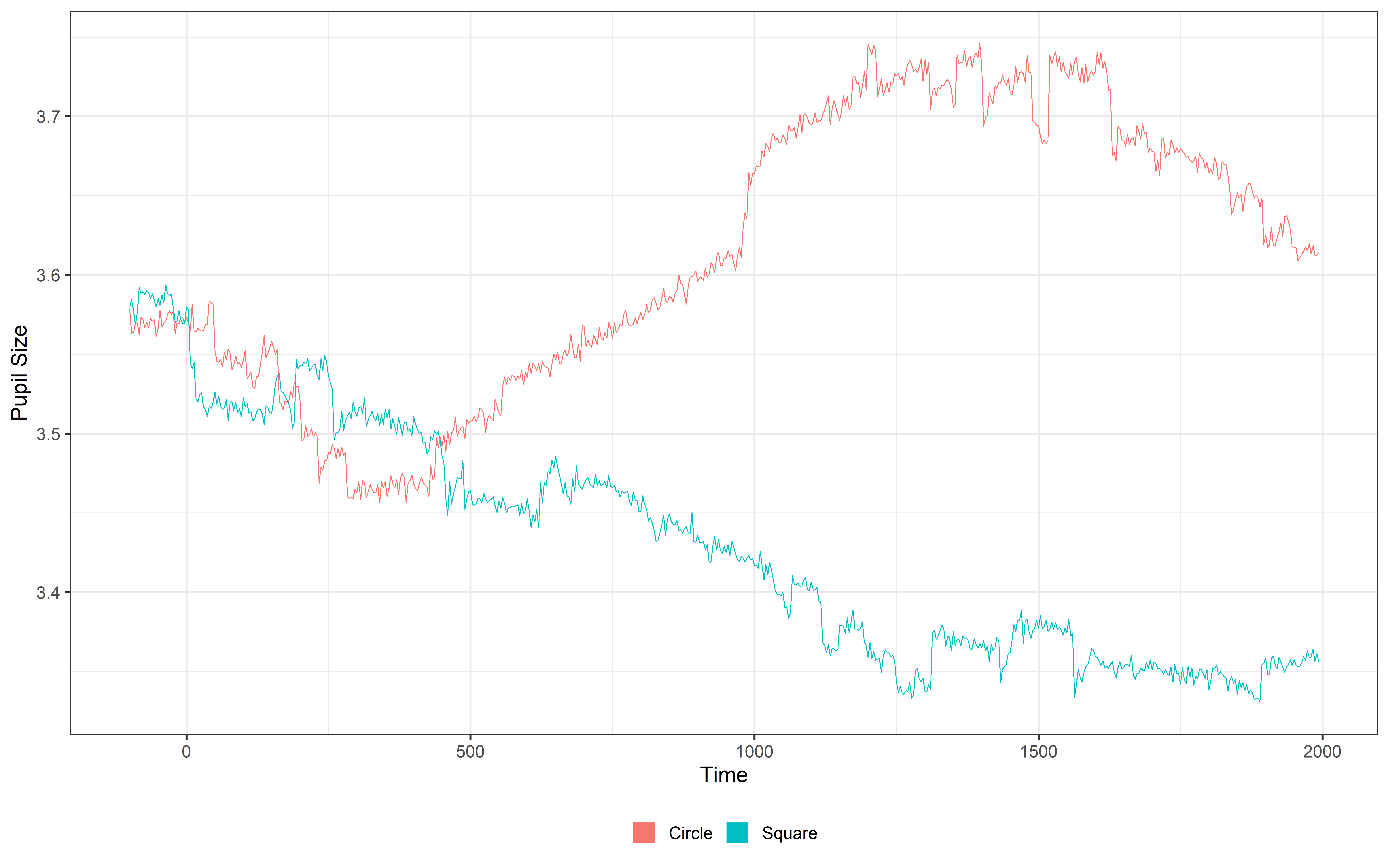
plot(Mean_data, pupil = mean_pupil, group = 'condition', geom = 'line')+
theme_bw(base_size = 45) +
theme(
legend.position = 'bottom',
legend.title = element_blank()) +
guides(color = guide_legend(override.aes = list(lwd = 20))) Lowpass
Now that we have a single pupil signal, we can move on to filtering it. The goal here is to remove fast noise and fluctuations that aren’t relevant to our analysis. Why? Because we know that pupil dilation is a slow physiological signal, and those rapid changes are likely just noise from blinks, eye movements, or measurement errors. By filtering out these fast fluctuations, we can focus on the meaningful changes in pupil dilation that matter for our analysis.
Filtered_data = filter_data(data = Mean_data,
pupil = mean_pupil,
filter = 'median',
degree = 11)
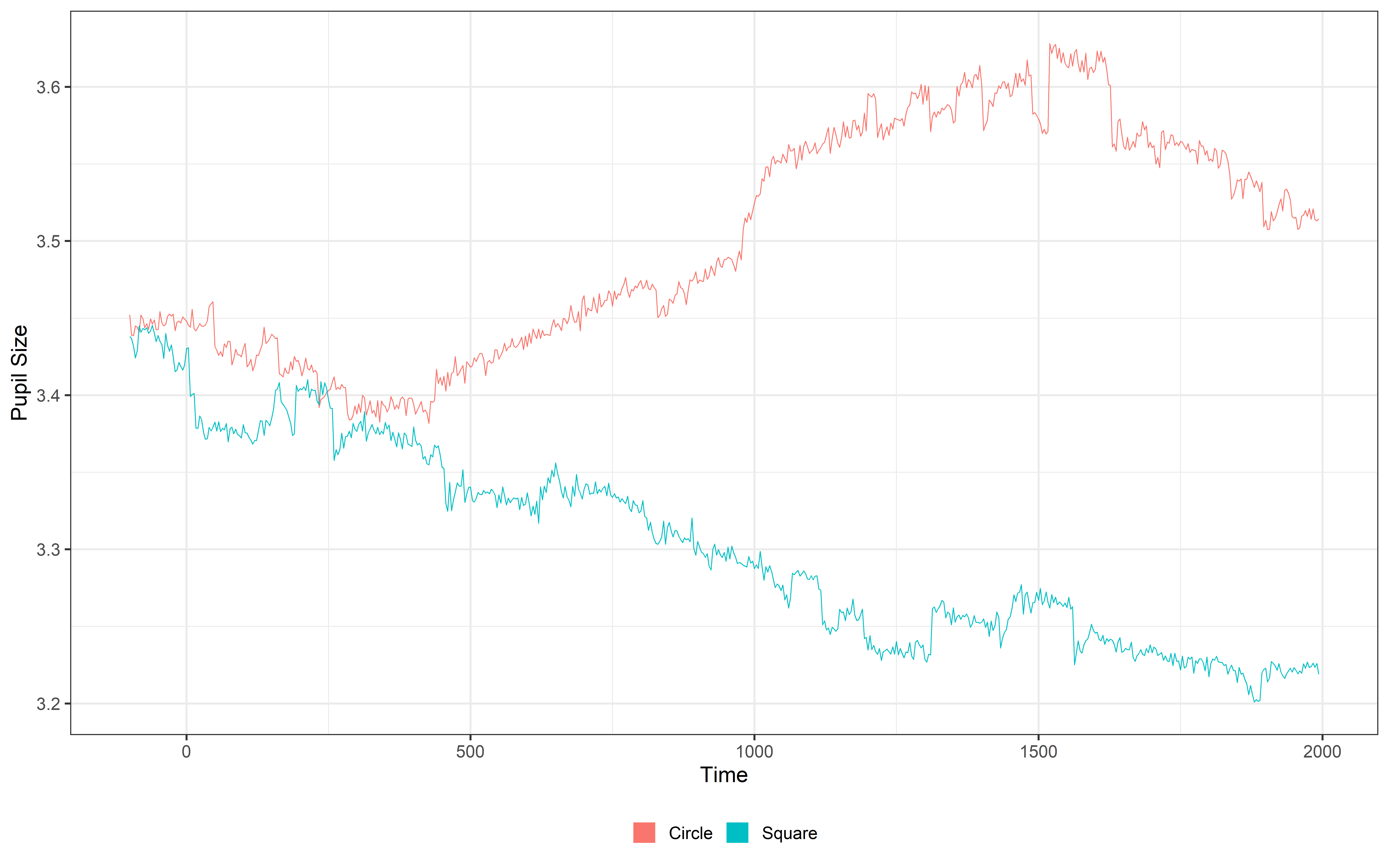
plot(Filtered_data, pupil = mean_pupil, group = 'condition', geom = 'line')+
theme_bw(base_size = 45) +
theme(
legend.position = 'bottom',
legend.title = element_blank()) +
guides(color = guide_legend(override.aes = list(lwd = 20))) There are different ways to filter the data in PupillometryR we suggest you check the actual package website and make decision based on your data (filter_data). Here we use a median filter based on a 11 sample window.
Trial Rejection
Now that our data is smaller and smoother, it’s a good time to take a look at it. It doesn’t make sense to keep trials that are mostly missing values, nor does it make sense to keep participants with very few good trials.
While you might already have info on trial counts and participant performance from other sources (like video coding), PupillometryR has a super handy function to check this directly. This way, you can quickly see how many valid trials each participant has and decide which ones to keep or drop.
Missing_data = calculate_missing_data(Filtered_data,
mean_pupil)
head(Missing_data, n=20)# A tibble: 20 × 3
Subject TrialN Missing
<chr> <int> <dbl>
1 Subject_1 2 0.0603
2 Subject_1 3 0.125
3 Subject_1 4 0.0746
4 Subject_1 5 0.106
5 Subject_1 6 0.0746
6 Subject_1 7 0.0635
7 Subject_1 8 0.0587
8 Subject_1 9 0.0619
9 Subject_1 10 0.130
10 Subject_2 1 0.143
11 Subject_2 2 0.121
12 Subject_2 3 0.0619
13 Subject_2 4 0
14 Subject_2 5 0.132
15 Subject_2 6 0.137
16 Subject_2 7 0.0841
17 Subject_2 8 0.0968
18 Subject_2 9 0.0841
19 Subject_2 10 0.0508
20 Subject_3 1 0.0587This gives us a new dataframe that shows the amount of missing data for each subject and each trial. While we could manually decide which trials and subjects to keep or remove, PupillometryR makes it easier with the clean_missing_data() function.
This function lets you set two % thresholds — one for trials and one for subjects. Here, we’ll set it to reject trials with more than 25% missing data (keep at least 75% of the data) and reject subjects with more than 25% missing data. This way, we ensure our analysis is based on clean, high-quality data.
Clean_data = clean_missing_data(Filtered_data,
pupil = mean_pupil,
trial_threshold = .75,
subject_trial_threshold = .75)Removing trials with a proportion missing > 0.75
...removed 3 trials Removing subjects with a proportion of missing trials > 0.75
...removed 0 subjects See?! PupillometryR shows us exactly how many trials and subjects are being excluded from our dataframe based on our thresholds. Cool!
Note that this function calculates the percentage of missing trials based only on the trials present in the dataframe. For example, if a participant only completed one trial (and watched it perfectly) before the session had to stop, the percentage would be calculated on that single trial, and the participant wouldn’t be rejected.
If you have more complex conditions for excluding participants (e.g., based on total expected trials or additional criteria), you’ll need to handle this manually to ensure subjects are dropped appropriately.
Fill the signal
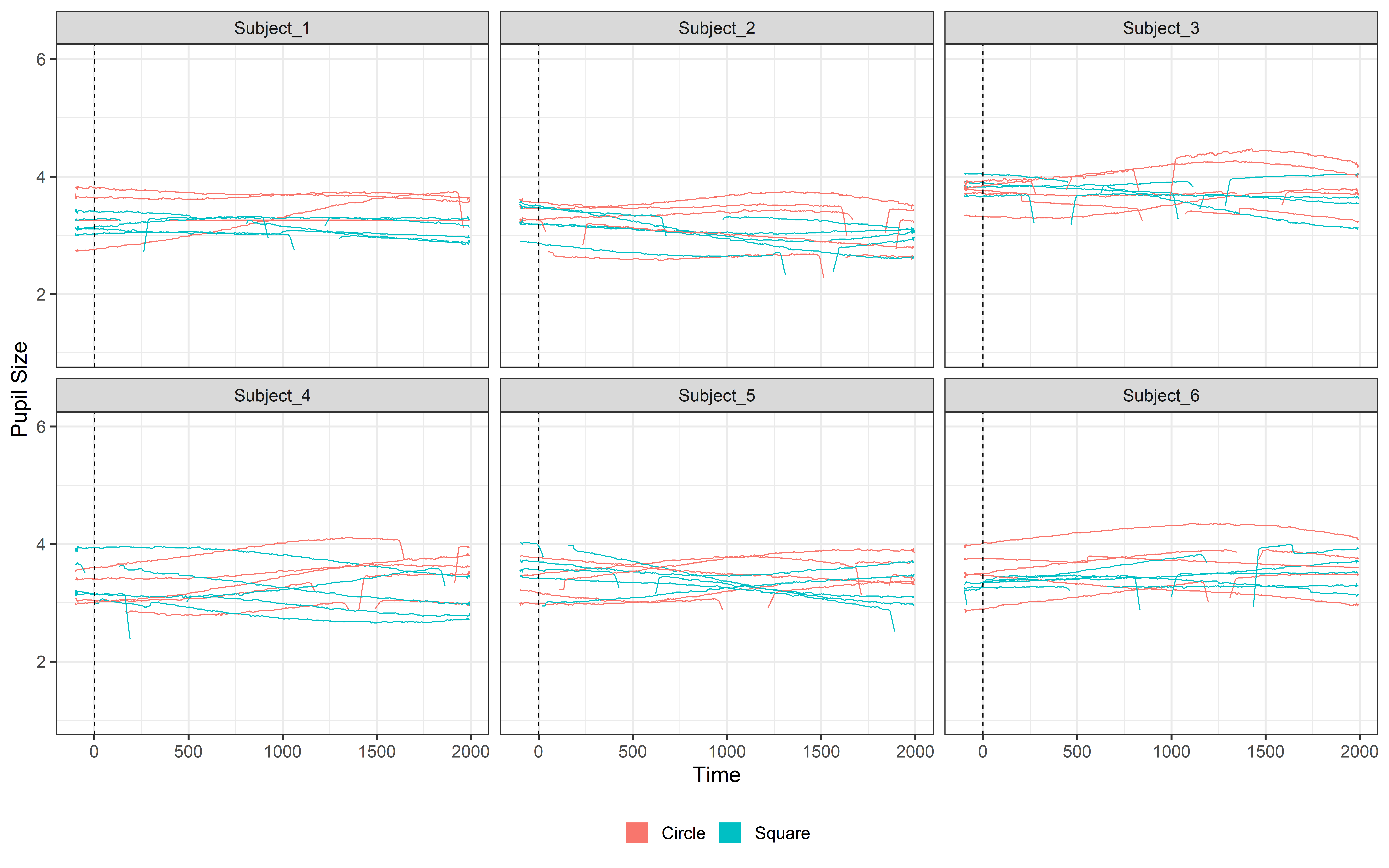
Now our data is clean, but… while the average signal for each condition looks smooth (as seen in our plots), the data for each individual participant is still noisy. We can still spot blinks and missing data in the signal.
To handle this, we’ll use interpolation to fill in the missing points. Interpolation “connects the dots” between gaps, creating a more continuous and cleaner signal. This step is crucial because large chunks of missing data can distort our analysis, and interpolation allows us to retain more usable data from each participant.
ggplot(Clean_data, aes(x = time, y = mean_pupil, group = TrialN, color= Event))+
geom_line( lwd =1.2)+
geom_vline(aes(xintercept = 0), linetype= 'dashed', color = 'black', lwd =1.2)+
facet_wrap(~Subject)+
ylim(1,6)+
theme_bw(base_size = 45) +
theme(
legend.position = 'bottom',
legend.title = element_blank()) +
labs(y = 'Pupil Size')+
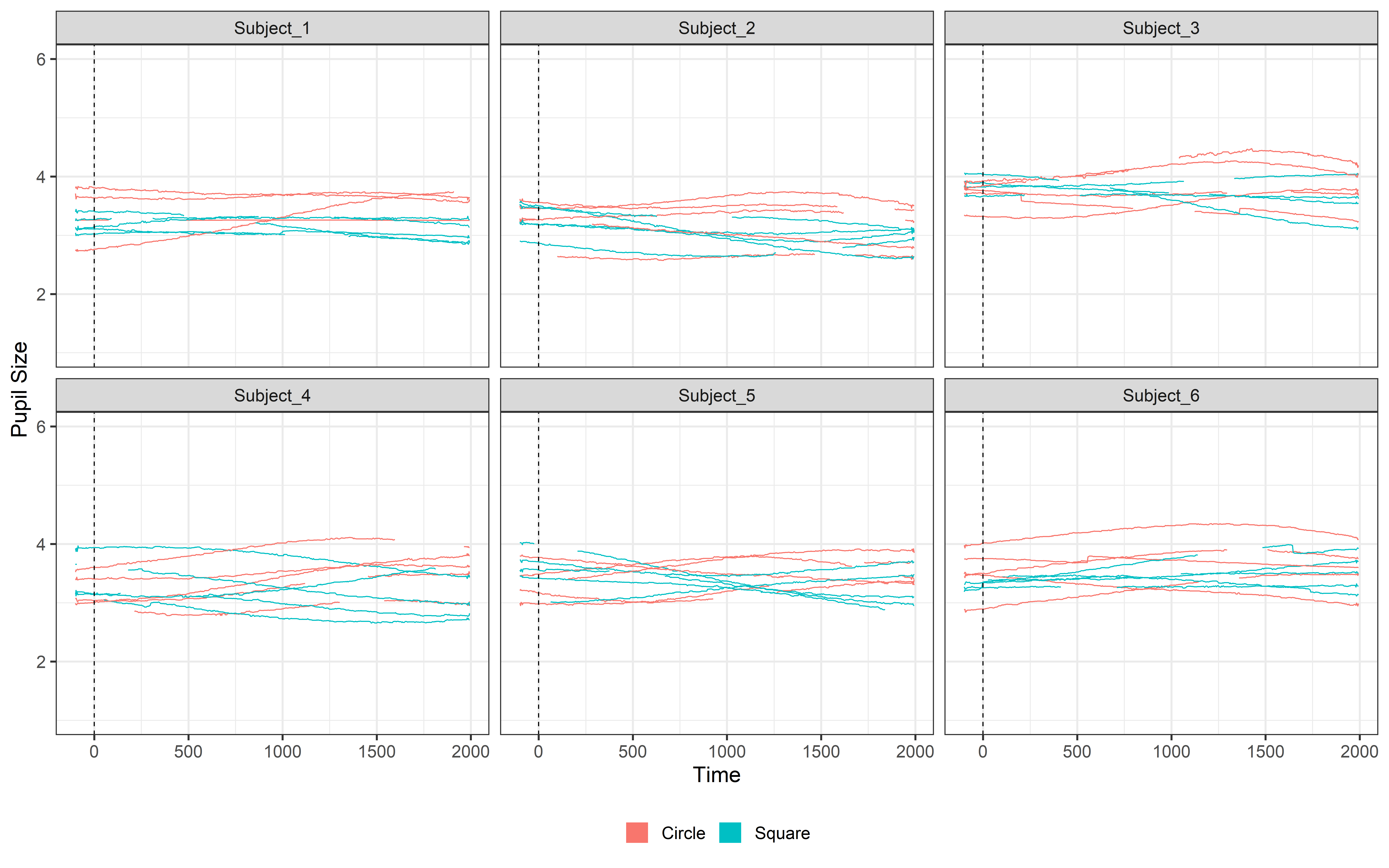
guides(color = guide_legend(override.aes = list(lwd = 20))) So to remove these missing values we can interpolate our data. Interpolating is easy with PupillometryR we can simply:
Int_data = interpolate_data(data = Clean_data,
pupil = mean_pupil,
type = 'linear')
ggplot(Int_data, aes(x = time, y = mean_pupil, group = TrialN, color = Event))+
geom_line(lwd =1.2)+
geom_vline(aes(xintercept = 0), linetype= 'dashed', color = 'black', lwd =1.2)+
facet_wrap(~Subject)+
ylim(1,6)+
theme_bw(base_size = 45) +
theme(
legend.position = 'bottom',
legend.title = element_blank()) +
labs(y = 'Pupil Size')+
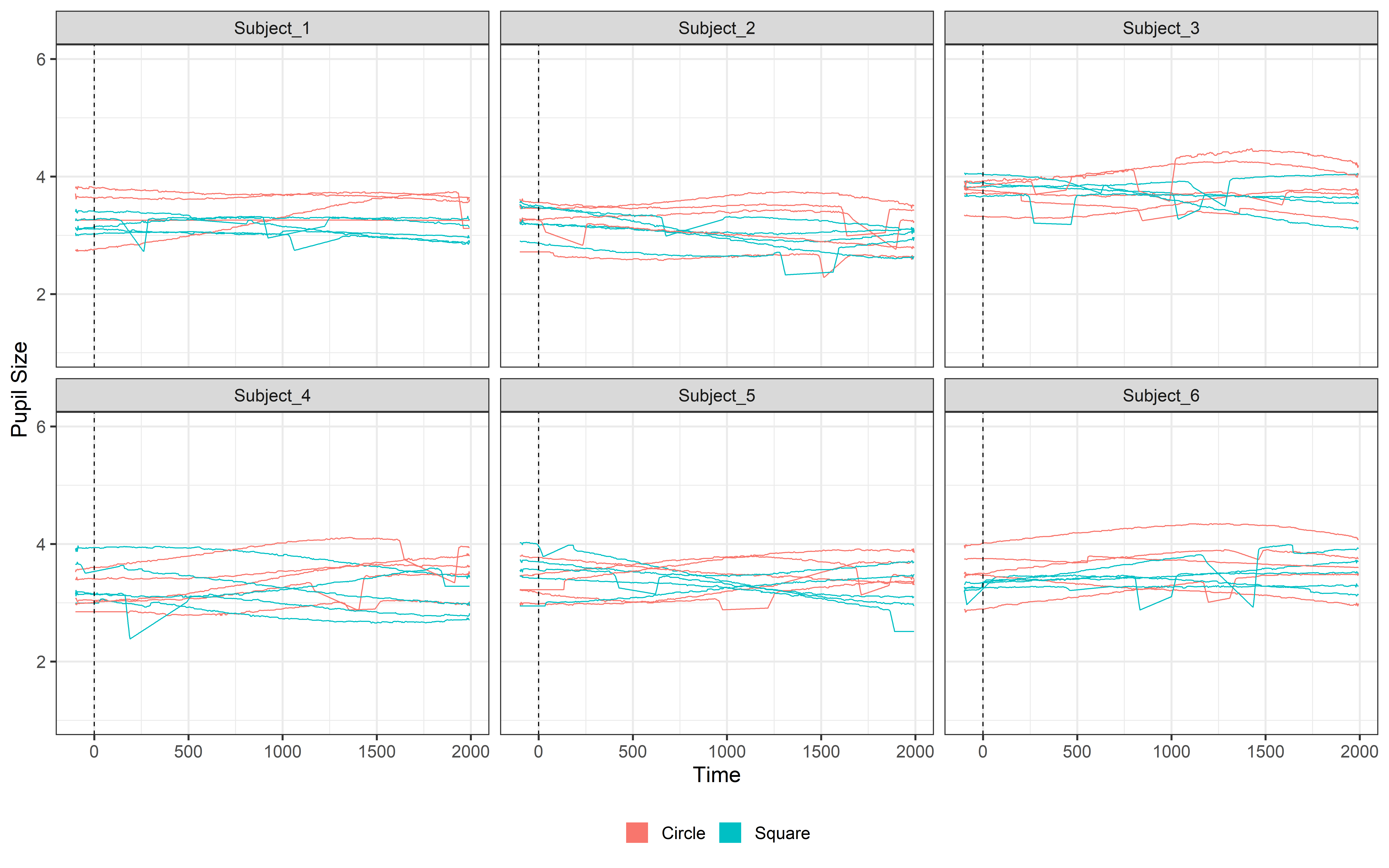
guides(color = guide_legend(override.aes = list(lwd = 20))) Done!! Well, you’ve probably noticed something strange… When there’s a blink, the pupil signal can rapidly decrease until it’s completely missing. Right now, this drop gets interpolated, and the result is a weird, unrealistic curve where the signal dips sharply and then smoothly recovers. This makes our data look horrible! 😩
Let’s fix it!
To do this, we’ll use PupillometryR’s blink detection functions. There are two main ways to detect blinks:
Based on size — detects pupil size.
Based on velocity — detects rapid changes in pupil size (which happens during blinks).
Here, we’ll use detection by velocity. We set a velocity threshold to detect when the pupil size changes too quickly. To ensure we capture the full blink, we use extend_forward and extend_back to expand the blink window, including the fast decrease in pupil size. The key idea is to make the entire blink period NA, not just the moment the pupil disappears. This prevents interpolation from creating unrealistic artifacts. When we interpolate, the process skips over the entire blink period, resulting in a cleaner, more natural signal.
Blink_data = detect_blinks_by_velocity(
Clean_data,
mean_pupil,
threshold = 0.1,
extend_forward = 70,
extend_back = 70)
ggplot(Blink_data, aes(x = time, y = mean_pupil, group = TrialN, color=Event))+
geom_line(lwd =1.2)+
geom_vline(aes(xintercept = 0), linetype= 'dashed', color = 'black', lwd =1.2)+
facet_wrap(~Subject)+
ylim(1,6)+
theme_bw(base_size = 45) +
theme(
legend.position = 'bottom',
legend.title = element_blank()) +
labs(y = 'Pupil Size')+
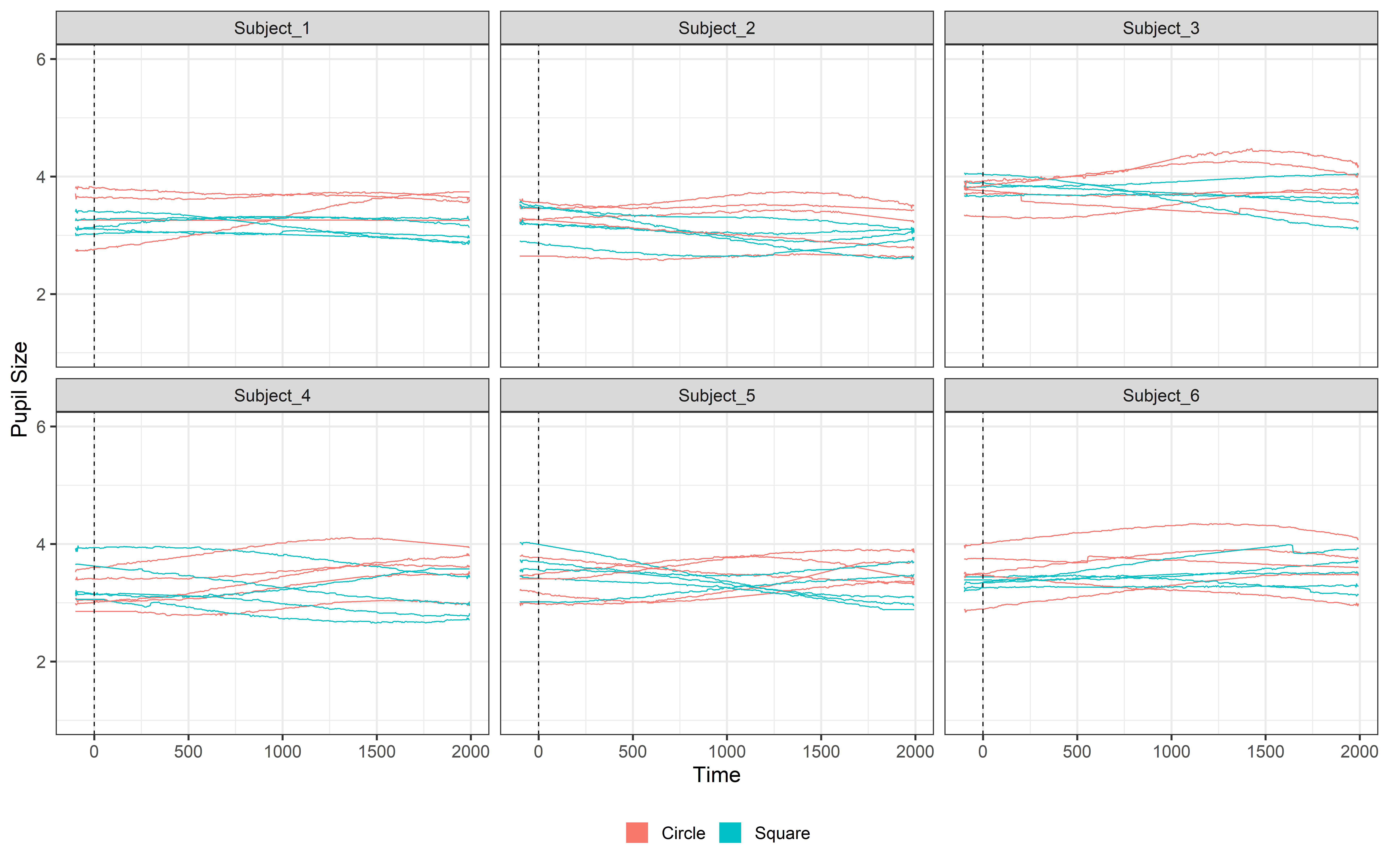
guides(color = guide_legend(override.aes = list(lwd = 20))) See !! now the rapid shrinking disappeared and we can now interpolate
Int_data = interpolate_data(data = Blink_data,
pupil = mean_pupil,
type = 'linear')
ggplot(Int_data, aes(x = time, y = mean_pupil, group = TrialN, color=Event))+
geom_line(lwd =1.2)+
geom_vline(aes(xintercept = 0), linetype= 'dashed', color = 'black', lwd =1.2)+
facet_wrap(~Subject)+
ylim(1,6)+
theme_bw(base_size = 45) +
theme(
legend.position = 'bottom',
legend.title = element_blank()) +
labs(y = 'Pupil Size')+
guides(color = guide_legend(override.aes = list(lwd = 20))) Look how beautiful our signal is now!! 😍 Good job!!!
You won’t always run into blink issues like this. Downsampling and filtering usually handle rapid changes during earlier preprocessing steps. Whether this happens can depend on the tracker, sampling rate, or even the population you’re testing. In this simulated data, we exaggerated the blink effects on purpose to show you how to spot and fix them! Thus, blink detection may not always be necessary. The best approach is to check your data before deciding. And how do you check it? Plotting! Plotting your signal is the best way to see if blinks are causing rapid drops or if you’re just dealing with missing data. Let the data guide your decisions.
Downsample
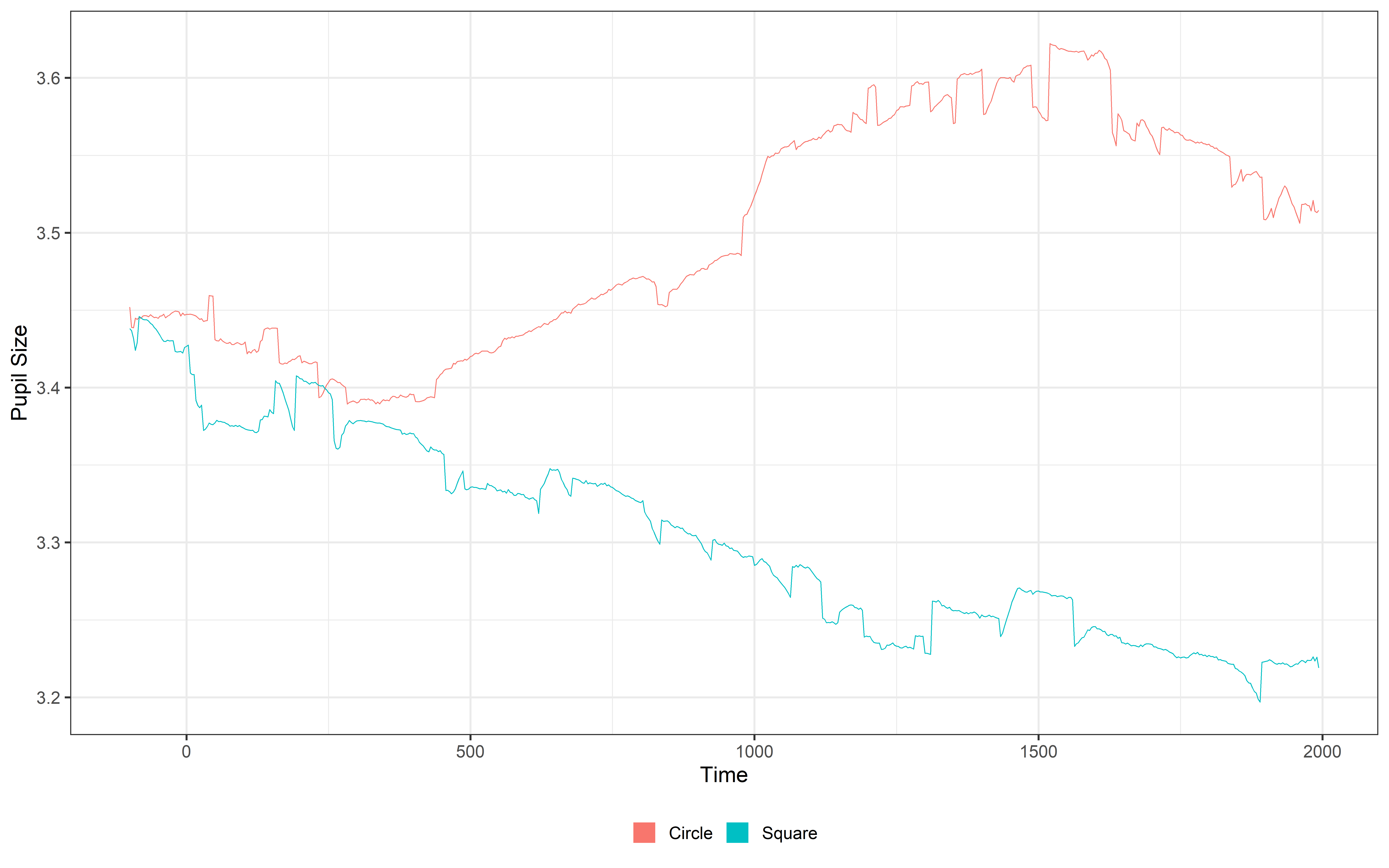
As mentioned before, Pupil dilation is a slow signal, so 20Hz is enough — no need for 300Hz. Downsampling reduces file size, speeds up processing, and even naturally smooths the signal, all while preserving the key information we need for analysis. To downsample to 20Hz, we’ll set the timebin size to 50 ms (since 1000/20 = 0.05 seconds = 50 ms) and calculate the median for each time bin.
NewHz = 20
timebinSize = 1000/NewHz
Downsampled_data = downsample_time_data(data = Int_data,
pupil = mean_pupil,
timebin_size = timebinSize,
option = 'median')
plot(Downsampled_data, pupil = mean_pupil, group = 'condition', geom = 'line') +
theme_bw(base_size = 45) +
theme(
legend.position = 'bottom',
legend.title = element_blank()) +
guides(color = guide_legend(override.aes = list(lwd = 20))) Baseline Correction
Good job getting this far!! We’re now at the final step of our pre-processing: baseline correction.
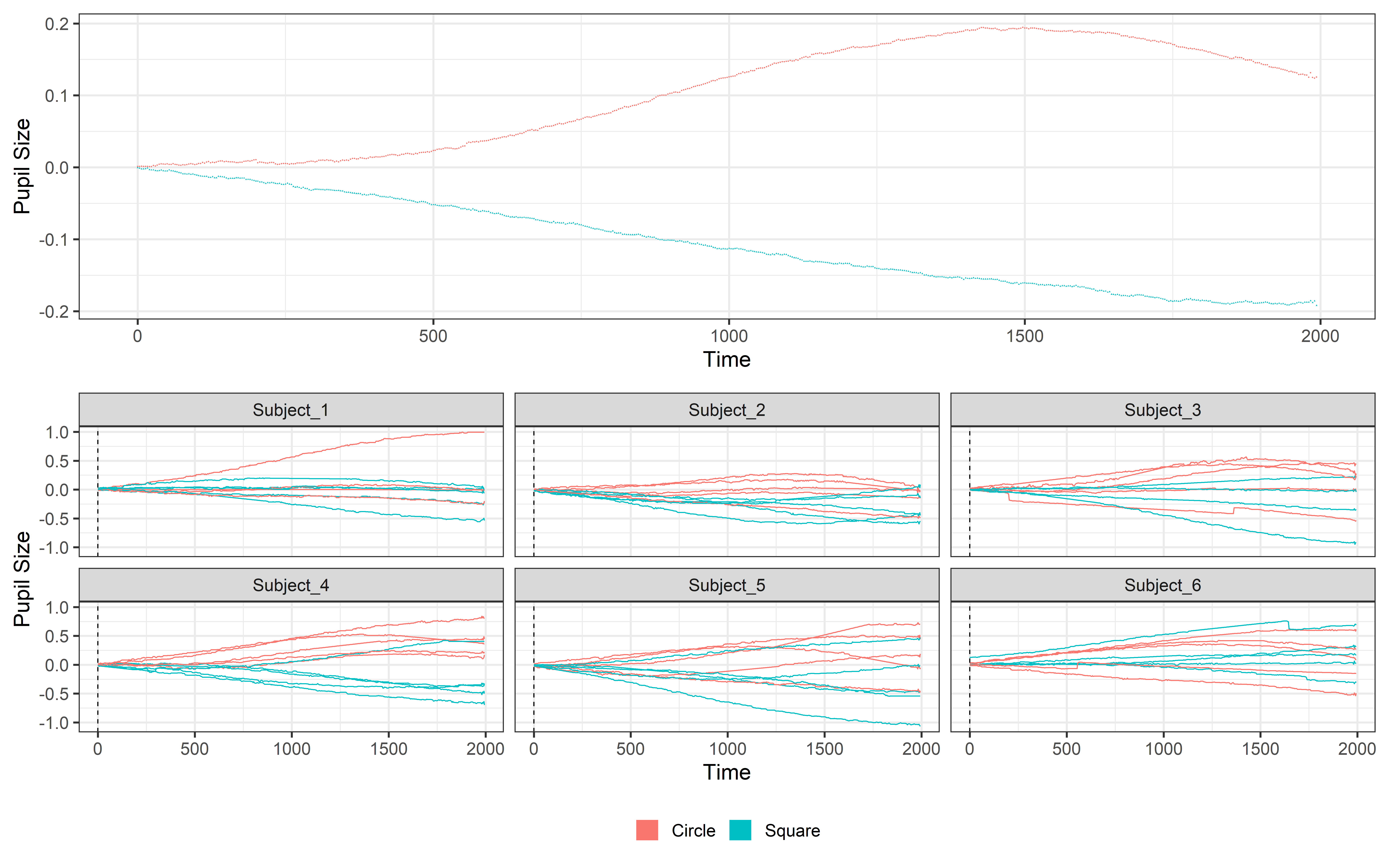
Baseline correction helps remove variability between trials and participants, like differences in baseline pupil size caused by individual differences, fatigue, or random fluctuations. By doing this, we can focus only on the variability caused by our paradigm. This step ensures that any changes we see in pupil size are truly driven by the experimental conditions, not irrelevant noise. To further adjust the data, we’ll subtract the calculated baseline, ensuring the values start at 0 instead of -100. Finally, to make the next steps of analysis easier, we’ll select only the columns of interest, dropping any irrelevant ones.
Let’s get it done!
Base_data = baseline_data(data = Downsampled_data,
pupil = mean_pupil,
start = -100,
stop = 0)
# Remove the baseline
Final_data = subset_data(Base_data, start = 0) %>%
select(Subject, Event, TrialN, mean_pupil, time)Let’s plot it to see what baseline correction and removal are actually doing!! We will plot both the average signal using the plot function (with some addition information about color and theme) and using ggplot to plot the data for each subject separately.
One = plot(Final_data, pupil = mean_pupil, group = 'condition', geom = 'line')+
theme_bw(base_size = 45) +
theme(legend.position = 'none')
Two = ggplot(Final_data, aes(x = time, y = mean_pupil, group = TrialN, color = Event))+
geom_line(lwd =1.2)+
geom_vline(aes(xintercept = 0), linetype= 'dashed', color = 'black', lwd =1.2)+
facet_wrap(~Subject)+
theme_bw(base_size = 45) +
theme(
legend.position = 'bottom',
legend.title = element_blank()) +
labs(y = 'Pupil Size')+
guides(color = guide_legend(override.aes = list(lwd = 20)))
# Using patchwork to put the plot together
One / TwoSave and analysis
This tutorial will not cover the analysis of pupil dilation. We’ll stop here since, after baseline correction, the data is ready to be explored and analyzed. From this point on, we’ll shift from pre-processing to analysis, so it’s a good idea to save the data as a simple .csv file for easy access and future use.
write.csv(Final_data, "..\\..\\resources\\Pupillometry\\Processed\\Processed_PupilData.csv")There are multiple ways to analyze pupil data, and we’ll show you some of our favorite methods in a dedicated tutorial: Analyze Pupil Dilation.
Cite PupillometryR
If you decide to use PupillometryR in your analysis, don’t forget to cite it! Proper citation acknowledges the authors’ work and supports the development of such valuable tools.
Code
citation("PupillometryR")To cite PupillometryR in publications use:
Forbes, S. H. (2020). PupillometryR: An R package for preparing and
analysing pupillometry data. Journal of Open Source Software, 5(50),
2285. https://doi.org/10.21105/joss.02285
A BibTeX entry for LaTeX users is
@Article{,
title = {PupillometryR: An R package for preparing and analysing pupillometry data},
author = {Samuel H. Forbes},
journal = {Journal of Open Source Software},
year = {2020},
volume = {5},
number = {50},
pages = {2285},
doi = {10.21105/joss.02285},
}All code
Here below we report the whole code we went trough this tutorial as an unique script to make it easier for you to copy and explore it in it’s entirety.
# Libraries and files --------------------------------------------------------------------
library(PupillometryR) # Library to process pupil signal
library(tidyverse) # Library to wrangle dataframes
library(patchwork)
csv_files = list.files(
path = "..\\..\\resources\\Pupillometry\\RAW",
pattern = "\\.csv$", # regex pattern to match .csv files
full.names = TRUE # returns the full file paths
)
# Prepare data --------------------------------------------------------------------
## Event settings --------------------------------------------------------------------
# Settings to cut events
Fs = 300 # framerate
Step = 1000/Fs
Pre_stim = 100 # pre stimulus time (100ms)
Post_stim = 2000 # post stimulus time (2000ms)
Pre_stim_samples = Pre_stim/Step # pre stimulus in samples
Post_stim_samples = Post_stim/Step # post stimulus in samples
# Time vector based on the event duration
Time = seq(from = -Pre_stim, by=Step, length.out = (Pre_stim+Post_stim)/Step) # time vector
## Event fixes --------------------------------------------------------------------
List_of_subject_dataframes = list() # Empty list to be filled with dataframes
# Loop for each subject
for (sub in 1:length(csv_files)) {
Raw_data = read.csv(csv_files[sub]) # Raw data
Events = filter(Raw_data, Event %in% Events_to_keep) # Events
# Loop for each event
for (trial in 1:nrow(Events)){
# Extract the information
Event = Events[trial,]$Event
TrialN = Events[trial,]$TrialN
# Event onset information
Onset = Events[trial,]$time
Onset_index = which.min(abs(Raw_data$time - Onset))
# Find the rows to update based on pre post samples
rows_to_update = seq(Onset_index - Pre_stim_samples,
Onset_index + Post_stim_samples-1)
# Repeat the values of interest for all the rows
Raw_data[rows_to_update, 'time'] = Time
Raw_data[rows_to_update, 'Event'] = Event
Raw_data[rows_to_update, 'TrialN'] = TrialN
}
# Filter only events of interest
Trial_data = Raw_data %>%
filter(Event %in% Events_to_keep)
# Add daframe to list
List_of_subject_dataframes[[sub]] = Trial_data
}
# Combine the list of dataframes into 1 dataframe
Trial_data = bind_rows(List_of_subject_dataframes)
### Plot Raw Data -----------------------------------------------------------------
ggplot(Raw_data, aes(x = time, y = R_P)) +
geom_line(aes(y = R_P, color = 'Pupil Right'), lwd = 1.2) +
geom_line(aes(y = L_P, color = 'Pupil Left'), lwd = 1.2) +
geom_vline(data = Raw_data |> dplyr::filter(!is.na(Event)), aes(xintercept = time, linetype = Event), lwd = 1.3) +
theme_bw(base_size = 45) +
ylim(1, 6) +
labs(color= 'Signal', y='Pupil size')+
scale_color_manual(
values = c('Pupil Right' = '#4A6274', 'Pupil Left' = '#E2725A') ) +
theme(
legend.position = 'bottom' ) +
guides(
color = guide_legend(override.aes = list(lwd = 20)),
linetype = guide_legend(override.aes = list(lwd = 1.2))
)
# Pre-processing -----------------------------------------------------------------
## Filter Out Trials with all NA -----------------------------------------------------------------
Trial_data = Trial_data %>%
group_by(Subject, TrialN) %>%
filter(!all(is.na(L_P) & is.na(R_P))) %>%
ungroup()
## Make PupillometryR Data -----------------------------------------------------------------
PupilR_data = make_pupillometryr_data(data = Trial_data,
subject = Subject,
trial = TrialN,
time = time,
condition = Event)
### Plot ------------------------------------------------------------------
plot(PupilR_data, pupil = L_P, group = 'condition', geom = 'line') +
theme_bw(base_size = 45) +
theme(
legend.position = 'bottom',
legend.title = element_blank()) +
guides(color = guide_legend(override.aes = list(lwd = 20)))
## Regress Data -----------------------------------------------------------------
Regressed_data = regress_data(data = PupilR_data,
pupil1 = L_P,
pupil2 = R_P)
## Calculate Mean Pupil -----------------------------------------------------------------
Mean_data = calculate_mean_pupil_size(data = Regressed_data,
pupil1 = L_P,
pupil2 = R_P)
### Plot --------------------------------------------------------------------
plot(Mean_data, pupil = mean_pupil, group = 'condition', geom = 'line')+
theme_bw(base_size = 45) +
theme(
legend.position = 'bottom',
legend.title = element_blank()) +
guides(color = guide_legend(override.aes = list(lwd = 20)))
## Lowpass Filter -----------------------------------------------------------------
filtered_data = filter_data(data = Mean_data,
pupil = mean_pupil,
filter = 'median',
degree = 11)
### Plot --------------------------------------------------------------------
plot(filtered_data, pupil = mean_pupil, group = 'condition', geom = 'line')+
theme_bw(base_size = 45) +
theme(
legend.position = 'bottom',
legend.title = element_blank()) +
guides(color = guide_legend(override.aes = list(lwd = 20)))
## Downsample -----------------------------------------------------------------
NewHz = 20
timebinSize = 1 / NewHz
Downsampled_data = downsample_time_data(data = filtered_data,
pupil = mean_pupil,
timebin_size = timebinSize,
option = 'median')
# Plot --------------------------------------------------------------------
plot(Downsampled_data, pupil = mean_pupil, group = 'condition', geom = 'line') +
theme_bw(base_size = 45) +
theme(
legend.position = 'bottom',
legend.title = element_blank()) +
guides(color = guide_legend(override.aes = list(lwd = 20)))
## Calculate Missing Data -----------------------------------------------------------------
Missing_data = calculate_missing_data(Downsampled_data, mean_pupil)
## Clean Missing Data -----------------------------------------------------------------
Clean_data = clean_missing_data(Downsampled_data,
pupil = mean_pupil,
trial_threshold = .75,
subject_trial_threshold = .75)
### Plot --------------------------------------------------------------------
ggplot(Clean_data, aes(x = Time, y = mean_pupil, group = TrialN, color= Event))+
geom_line( lwd =1.2)+
geom_vline(aes(xintercept = 0), linetype= 'dashed', color = 'black', lwd =1.2)+
facet_wrap(~Subject)+
ylim(1,6)+
theme_bw(base_size = 45) +
theme(
legend.position = 'bottom',
legend.title = element_blank()) +
guides(color = guide_legend(override.aes = list(lwd = 20)))
## Detect Blinks -----------------------------------------------------------------
Blink_data = detect_blinks_by_velocity(
Clean_data,
mean_pupil,
threshold = 0.1,
extend_forward = 50,
extend_back = 50)
### Plot --------------------------------------------------------------------
ggplot(Blink_data, aes(x = time, y = mean_pupil, group = TrialN, color=Event))+
geom_line(lwd =1.2)+
geom_vline(aes(xintercept = 0), linetype= 'dashed', color = 'black', lwd =1.2)+
facet_wrap(~Subject)+
ylim(1,6)+
theme_bw(base_size = 45) +
theme(
legend.position = 'bottom',
legend.title = element_blank()) +
guides(color = guide_legend(override.aes = list(lwd = 20)))
## Interpolate Data -----------------------------------------------------------------
Int_data = interpolate_data(data = Clean_data,
pupil = mean_pupil,
type = 'linear')
### Plot --------------------------------------------------------------------
ggplot(Int_data, aes(x = Time, y = mean_pupil, group = TrialN, color = Event))+
geom_line(lwd =1.2)+
geom_vline(aes(xintercept = 0), linetype= 'dashed', color = 'black', lwd =1.2)+
facet_wrap(~Subject)+
ylim(1,6)+
theme_bw(base_size = 45) +
theme(
legend.position = 'bottom',
legend.title = element_blank()) +
guides(color = guide_legend(override.aes = list(lwd = 20)))
# Baseline correction -----------------------------------------------------
Base_data = baseline_data(data = Int_data,
pupil = mean_pupil,
start = -100,
stop = 0)
# Remove the baseline
Final_data = subset_data(Base_data, start = 0)
### Final plot --------------------------------------------------------------
One = plot(Final_data, pupil = mean_pupil, group = 'condition')+
theme_bw(base_size = 45) +
theme(legend.position = 'none')
Two = ggplot(Final_data, aes(x = time, y = mean_pupil, group = TrialN, color = Event))+
geom_line(lwd =1.2)+
geom_vline(aes(xintercept = 0), linetype= 'dashed', color = 'black', lwd =1.2)+
facet_wrap(~Subject)+
theme_bw(base_size = 45) +
theme(
legend.position = 'bottom',
legend.title = element_blank()) +
guides(color = guide_legend(override.aes = list(lwd = 20)))
One / Two
# Save data ---------------------------------------------------------------
write.csv(Final_data, "..\\..\\resources\\Pupillometry\\Processed\\Peocessed_PupilData.csv")


